Mastering the Art of Creating Tables in Excel: A Step-by-Step Guide

Introduction

Tables are an incredibly powerful feature in Excel that not only organize data but also enhance their functionality and aesthetic appeal. Whether you're a student, a professional, or an entrepreneur, mastering the art of creating tables in Excel can revolutionize the way you work with data. In this blog post, we will take you through a step-by-step guide on how to create tables in Excel and unleash their full potential.

Step 1: Preparing your data: Before creating a table in Excel, it is vital to organize your data in a structured manner. Ensure that all your data is in one contiguous range with a single row for column headings. This will help maintain consistency and make your table easy to understand and navigate.

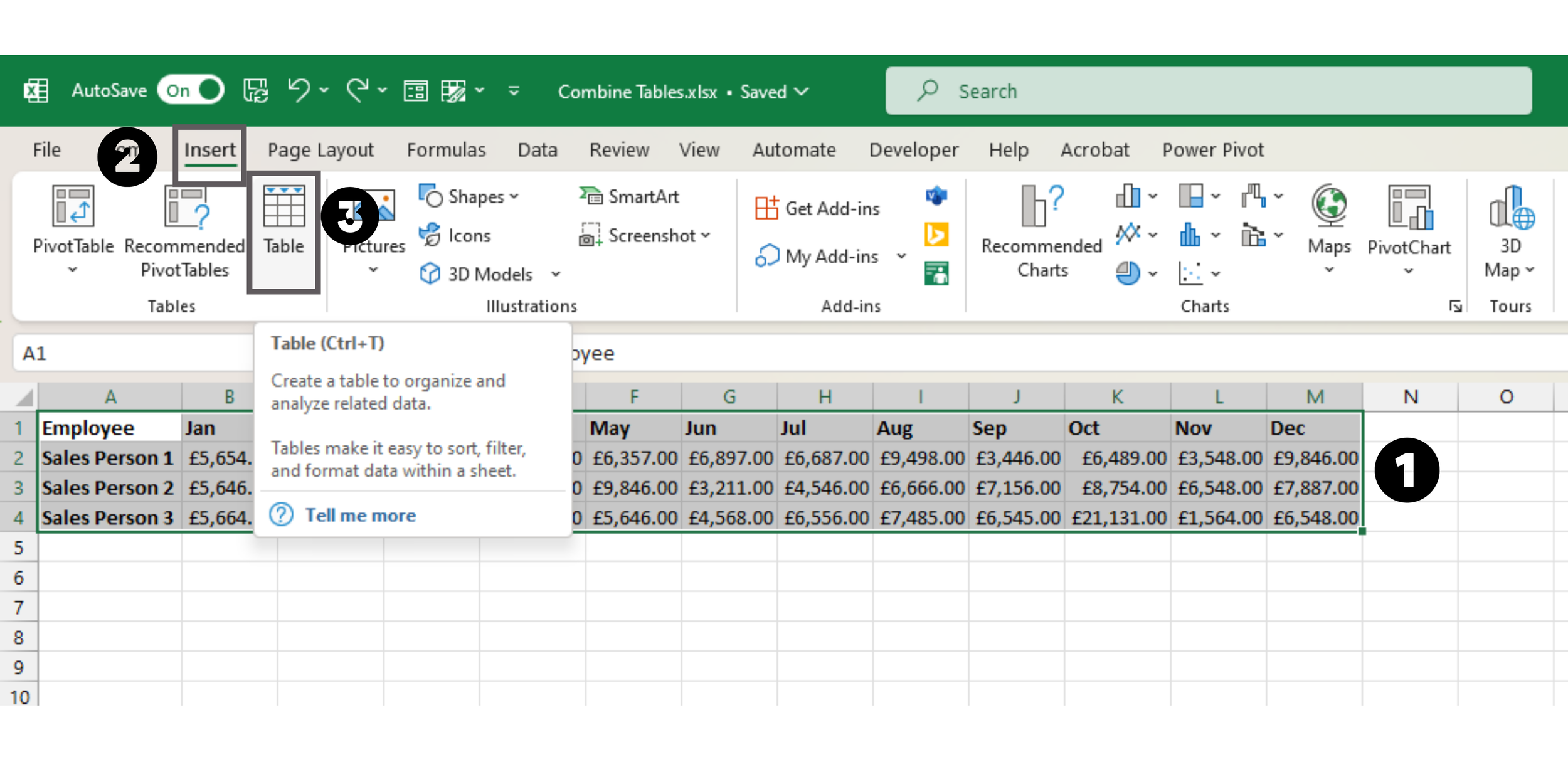
Step 2: Selecting your data and opening the Table dialog box: Now it's time to select your data range. Click and drag to highlight the desired range or use a combination of the Shift and Arrow keys to include multiple ranges. Once selected, navigate to the "Insert" tab on the ribbon. In the "Tables" group, click on the "Table" button.

Step 3: Verifying the range and naming your table: Excel will automatically detect the range you selected, and you should see a dialog box displaying the correct range. If required, you can adjust the range manually. Make sure the "My table has headers" box is checked to consider the first row as column headers.

Step 4: To rename your table in Microsoft Excel, simply go to the Name Box, usually found underneath the ribbon on the left-hand side next to the Formula Bar. Click on the Name Box and enter a new, descriptive name for your table. This allows for easier reference and improved organization within your Excel workbook. Press Enter to save the new name.

Step 5: Customizing the table style: Excel provides several built-in table styles to choose from. Selecting a suitable style can enhance the visual appeal of your table. Simply click on the "Table Styles" dropdown menu, located in the "Table Tools" contextual tab that appears once you have created a table. Experiment with different styles until you find the one that best suits your needs.

Step 6: Utilizing table features: Once you've created your table, a variety of powerful features become available to you. Here are a few key features to explore:

a) Filtering: Click on the filter arrow located in the header of each column to quickly sort, filter, and analyze data based on specific criteria.

b) Structured references: With tables, you can use structured references (e.g., [Jan) instead of cell references (e.g., B1:B4) when performing calculations or writing formulas. This allows for more readable and dynamic formulas.

c) Total Row: Enabling the Total Row option from the "Table Tools" tab adds a row at the end of the table, offering built-in formulas for summarizing data column-wise. You can choose from a variety of functions, such as sum, average, count, etc.

d) Data Validation: By applying data validation rules to specific columns, you can control and validate user-input or restrict entries to specific formats or ranges.

Conclusion:

Creating tables in Excel elevates your data management skills to a whole new level. Now that you know the step-by-step process, take advantage of this valuable feature and unlock the potential of your data. Excel tables enable improved organization, ease of filtering, and advanced calculations, empowering you to make data-driven decisions with efficiency. So, embrace the power of tables, and let Excel simplify your data analysis and reporting tasks like never before.